Building a 25M Parameter GPT from Scratch

“How hard can this be?”

To satisfy my curiosity and understand every design choice firsthand, I built a 25M parameter GPT from scratch. This article is a collection of the lessons I learned along the way.

TLDR

I trained a 25M parameter language model from scratch on 500M tokens from FineWeb and TinyStories, using modern architecture choices such as RoPE, GQA, SwiGLU, and RMSNorm. The final run used an NVIDIA RTX A5000 GPU for roughly two hours.

Model weights and logs are on Hugging Face. The training code is on GitHub.

Why bother building this?

Building a model from scratch taught me how much the pre-training data matters, gave me a more concrete intuition for scaling laws, and helped demystify a system that previously felt like a black box.

I was inspired by Karpathy’s NanoGPT. It made me think about how I could improve the architecture, try different dataset mixtures, and push for better results with fewer parameters and less compute. I wanted the repository to be easy for beginners to read while still being flexible enough for future experiments.

Section 1: Architecture

The earlier version LiteGPT-16M followed a GPT-2 style architecture with LayerNorm, multi-head attention, GELU feed-forward layers, and learned positional embeddings.

For the 25M model, I modernized the architecture with RMSNorm, SwiGLU, RoPE, and grouped-query attention. These choices make training faster and scale better.

Transformer architecture

1.1) Dataset

I started with a dataset mixture containing 60% Fineweb, 30% TinyStories and 10% The Stack Smol from HuggingFace because I wanted to fine-tune the base model later to create a small coding agent for fun but I had to remove the code dataset completely as I wanted the model to understand natural language better and the coding data introduced a very different token distribution than natural language and I thought that it would help the model generalize better.

The dataset I finally settled on and where the model was finally trained on was 60% FineWeb and 40% TinyStories. I expected the loss to go down by a lot after I removed the The Stack Smol dataset keeping only natural language data but this didn’t change the loss by too much.

Next experiment would be to train this model exclusively on FineWeb or TinyStories. I am quite sure I can get the model’s validation loss to go down.

Tokenizer

I initially used the GPT-2 tokenizer, the same one used in NanoGPT. I could not get validation loss below 4, which suggested something was fundamentally wrong.

The issue was vocabulary size. GPT-2’s vocabulary has 50,257 tokens. With d_model = 320, the embedding table alone used roughly 16M parameters out of the 25M total trainable parameters. That left too little capacity for the transformer itself.

To fix this, I trained a byte-level BPE tokenizer with a vocabulary size of about 16K using Hugging Face Tokenizers. The dataset is stored as uint16 binary files and loaded lazily with np.memmap(), which lets the data loader grab random chunks without loading the whole dataset into RAM.

500M tokens at uint16 is 500,000,000 x 2 bytes ~ 1GB

np.memmap() allows loading files bigger than the RAM and has a low startup time because it only loads the pages that are being read, directly from the disk.

1.2) Scaling laws

Before Chinchilla, models like GPT-3 were undertrained (175B params trained on ~300B tokens).

Chinchilla scaling laws suggest that for a fixed compute budget, model size and number of training tokens need to be balanced. The rough compute-optimal regime is about 20 training tokens per parameter.

For a 25M parameter model, that points toward roughly 500M training tokens. This is why I targeted a 500M-token dataset.

1.3) Learning rate schedule

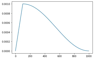
The learning rate linearly warms up to a peak of 6e-4 and then follows cosine decay. Warmup matters because early losses are large, and using a high learning rate immediately can make updates unstable. Cosine decay helps reduce update size as the model starts converging.

lr_graph

1.4) Transformer block

1.4.1) RMSNorm

The model uses a GPT-2 style pre-norm block, but with RMSNorm instead of LayerNorm. RMSNorm normalizes by root-mean-square magnitude and avoids subtracting the mean, which makes it cheaper than LayerNorm.

1.4.2) RoPE

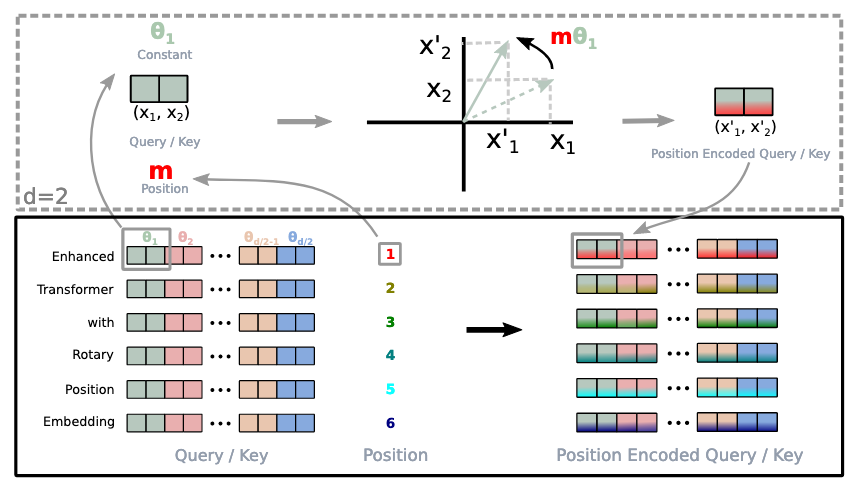
RoPE rotates the query and key vectors before attention, allowing the attention mechanism to model relative positions. I chose RoPE because it reduces learned positional parameters and tends to generalize better to longer contexts than learned positional embeddings.

rope

1.4.3) GQA

The attention block implements Grouped Query Attention (GQA), where there are n_heads query heads but only n_kv_heads key and value heads. Multiple query heads share the same key and value heads, significantly reducing the memory and computation required for the KV cache during inference.

Different attention heads learn different attention patterns. Empirical studies have shown that sharing keys and values across multiple query heads has little impact on model quality, making GQA an effective trade-off between efficiency and performance.

gqa

Attention is computed using torch.nn.functional.scaled_dot_product_attention(), which dispatches to highly optimized fused kernels that combine the attention operations into a single implementation, reducing memory accesses and improving throughput. When the hardware and input satisfy the required conditions, PyTorch automatically uses FlashAttention, providing further speedups and lower memory usage without requiring changes to the model code.

1.4.4) Residual add

After the attention block, the original input is added back to the output of the attention layer through a residual connection.

Residual connections preserve the original representation while providing an path for gradients, making optimization significantly easier. They provide a direct path for gradients to flow during backpropagation, helping avoid the vanishing gradient problem as models become deeper.

This allows each transformer block to learn a small refinement to the input instead of having to learn an entirely new representation from scratch, resulting in faster convergence and more stable training. The same residual connection is also applied after the SwiGLU feed-forward network, making every transformer block responsible for learning only incremental improvements to the representation.

1.4.5) SwiGLU MLP/FFN

Then comes the SwiGLU MLP, here, instead of one up-projection as done in GELU, there are 2 up-projections, one is the original up-projection and the other is the gate projection. This gating feature decides which features are worth keeping and which aren’t and suppresses those features thus acting as a feature gate.

1.4.6) Cross entropy loss

After going through n_layers of transformer blocks, it goes through a final RMSNorm and produces the final logits which are then passed through softmax to return probabilities over n_vocab choices.

The loss is calculated here using cross entropy loss which takes the negative log probability assigned to the correct next token.

The negative log is taken because it strongly penalizes when the model is confidently wrong. The farther the probability is from the correct answer, the stronger the penalty is.

1.4.7) Generation

The model doesn’t output probabilities by default, when the model is being used for inference, these logits are divided by the temperature and passed through a softmax function that gives us the probabilities of the next token over the entire vocabulary of the model.

Temperature controls the sharpness of the output probability distribution. Higher temperature produces a flatter distribution with more similar probabilities, while lower temperature produces a sharper distribution where the highest-probability tokens dominate.

Section 2: Implementation

This is the configuration of the model:

Parameter	Value
n_layers	8
batch_size	64
grad_accum_steps	2
d_model	448
n_heads	8
head_dim	56
n_kv_heads	4
ffn_dim	1152
context_length	512
vocab_size	16384

The hidden dimension follows the LLaMA-style rule of roughly 8 / 3 * d_model instead of the classic GPT-2 4 * d_model, because SwiGLU uses three linear projections rather than two.

Parameter count:

Component	Params
Token Embedding	16384 × 448 = 7,340,032
Attention (GQA)	[(448×448) + (448×224) + (448×224) + (448×448)] × 8 = 4,816,896
SwiGLU FFN	[(448×1152) + (448×1152) + (1152×448)] × 8 = 12,386,304
RMSNorm	(448 × 2) × 8 = 7,168
Final RMSNorm	448
LM Head	weight tied with token embeddings
Total	≈ 24.6M

Training ran for 40,000 forward and backward iterations with a gradient accumulation factor of 2, resulting in 20,000 optimizer steps.

The total number of tokens seen during training was:

64 x 512 x 40,000 = 1,310,720,000 tokens

That is about 1.3B tokens, or roughly 2.6 epochs over the 500M-token dataset.

Section 3: Issues I faced

3.1) Hardware constraints

I started on the free-tier T4 GPU on Google Colab, but it was too slow and sessions were terminated aggressively. The 16GB VRAM limit also forced a smaller batch size.

The memory used by a model in training is roughly:

Weights + Gradients + Optimizer states + Activation

I switched to RunPod and rented an NVIDIA RTX A5000, which let me increase batch size, hidden dimension, and other hyperparameters.

There are 2 ways to reduce the VRAM used on GPUs:

Gradient checkpointing: Instead of storing all the activations of the model, store only a few activations and when backpropagating, recompute the activations.
Gradient accumulation: This increases the effective batch size by accumulating gradients over multiple forward/backward passes before performing one optimizer update.

3.2) Loss not going down

The loss was not budging and the model was not able to get to a good loss value, which meant that something in my setup was broken.

After spending quite some time looking around I realized that my tokenizer had n_vocab of 50257 and the embedding layer ended up taking 16M params out of the 25M trainable ones and that’s why the model was just not able to generalize all that data when the transformer only had 9M params to train on.

3.3) Steps are not the right training metric

I initially thought training for more steps would automatically improve the model. That was wrong. The number of quality tokens seen during training is a much better thing to focus on.

For LiteGPT-16M, the training loss was around 2 while validation loss was around 5. That was a clear overfitting signal: the model memorized the training data but failed to generalize.

3.4) Wrong data mixture

The initial mix included coding data, but the model was too small to produce useful code. The code dataset also pulled the token distribution away from the natural language behavior I cared about most.

Section 4: Improvements to make

Train exclusively on FineWeb to test a larger and more diverse natural language distribution.
Scale to more than 1B tokens while following Chinchilla-style scaling laws.
Fine-tune on instruction data for a specific downstream task.
Try alternative optimizers such as AdamW-mini or Sophia.

Section 5: Example generations

Prompt: The capital of France is

well known for its great geographical experience. The historical setting is not one of a sort of the greatest of all the times, but it’s a central part of the history of the country. It’s a historical town that has seen a huge shift inside this famous city of the same name. The city is known as “The Dolceus” and also known as “The Dolceus.” It’s a place where a lot of people live and live.

Prompt: Once upon a time, there lived

a little girl named Lily. She was very excited because she was going on a trip to see Grandma. She helped her mom pack their luggage with clothes and toys. Then, they got in the car and drove to Grandma’s house. As they drove, Lily saw something strange. It was a big, gray cloud that seemed to float away. She pointed and asked her mom what it was. Her mom said it was a mild cloud, but it was a very hot day.

Prompt: The dragon opened its eyes and

looked around. It saw something shiny and colorful. It jumped and grabbed the object with its sharp claws. The dragon flew away and the dragon breathed a sigh of joy. It flew back up into the sky and found its owner, who was so proud of it. He said the dragon had been an amazing hunter.

Prompt: Tom had a little red ball.

Lily had a red ball and Tom had a blue ball. They both loved to play with their toys. But they both wanted the red ball. They both pulled it from each other. “Give me the red ball!” Lily shouted. “It’s mine!” “No, it’s mine!” Tom yelled. “It’s mine!” They pulled so hard that they separate the red ball from each other. They both fell down and started to cry. Mom heard the noise and came to see what was wrong. She saw the red ball on the floor and the tears on Lily’s face. She was not angry, but she was sad. “Why are you fighting?” Mom asked. “You both have the red ball, but you both have the same toy.” “That is boring!” Lily said. “You both need to share and take turns.” “Okay!” Mom said. “But you can both have the red ball.

Section 6: Results

Final metrics

Metric	Value
Train Loss	2.685
Val Loss	2.825
Perplexity	16.86

GPU Benchmark (Inference on A5000)

Metric	Value
Throughput	~75K tok/s
Latency (mean)	~4.2 ms
Latency (P95)	~5.8 ms
GPU Memory (alloc)	~0.9 GB

Section 7: Observations

The model performs best on story-like prompts, which is not surprising given the TinyStories mixture. Factual accuracy is poor at 25M parameters. Repetition loops become common at higher temperatures. Coding generations are essentially non-functional. Reasoning is limited, but the model does show a basic grasp of narrative structure.